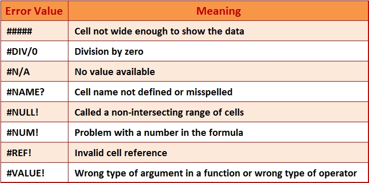
#####
This error indicates that a column is not wide enough to display all of its content, or that a negative date or time is used in a cell.
Causes
- The column is not wide enough to display the content.
- Dates and times are negative numbers.
Resolution
- Increase the width of the column to fit the text.
- Shrink the text size of the contents to fit the column
- Apply a different number or date format.
In some cases, you can change the number or date format of a cell to make its contents fit within the existing cell width. For example, you can decrease the number of decimal places after the decimal point or switch from a Long Date to a Short Date format.
- If you are using the 1900 date system, dates and times in Microsoft Excel must be positive values.
- When you subtract dates and times, make sure that you build the formula correctly.
- If a formula that you use to calculate dates or times is correct but results in a negative value, display that value in a format that is not a date or time format
#DIV/0!
Microsoft Excel displays the #DIV/0! error when a number is divided either by zero (0) or by a cell that contains no value.
Causes
- Entering a formula that performs explicit division by zero (0) - for example, =5/0.
- Using a reference to a blank cell or to a cell that contains zero as the divisor in a formula or function that performs division.
- Running a macro that uses a function or a formula that returns the #DIV/0! error.
Resolution
- Make sure that the divisor in the function or formula is not zero (0) or blank.
- Change the cell reference in the formula to another cell that does not contain a zero or a blank value.
- Enter the value #N/A in the cell that is referenced as the divisor in the formula.
Entering #N/A will change the result of the formula to #N/A from #DIV/0! to indicate that the divisor value is not available.
- Prevent the error value from being displayed by using the IF worksheet function. You can then display 0 or any string as the result.
For example, if the formula that produces the error is =A1/A2, use =IF(A2=0,"",A1/A2) to return an empty string, or =IF(A2=0,0,A1/A2) to return 0.
#N/A
This error indicates that a value is not available to a function or formula.
Causes
- Data is missing, and #N/A or NA() has been entered in its place.
- An inappropriate value was given for the lookup_value argument in the HLOOKUP, LOOKUP, MATCH, or VLOOKUP worksheet function.
- The VLOOKUP, HLOOKUP, or MATCH worksheet function was used to locate a value in an unsorted table.
- An array formula is using an argument that is not the same number of rows or columns as the range that contains the array formula.
- One or more required arguments were omitted from a built-in or custom worksheet function.
- A custom worksheet function that you use is not available.
- A macro that you run enters a function that returns #N/A.
Resolution
- Optionally, if error checking is turned on in Excel, click the button that appears next to the cell that displays the error, click Show Calculation Steps if it appears, and then click the resolution that is appropriate for your data.
Tip: Review the following resolutions to help determine which option to click.
- If you manually entered #N/A in a cell, replace it with actual data if that data is now available. For example, if you entered #N/A in cells where data is not yet available, formulas that refer to those cells also return #N/A instead of attempting to calculate a value. If you enter a value instead, the error should be resolved in the cells that contain the formulas.
- Make sure that the lookup_value argument that you entered in a HLOOKUP, LOOKUP, MATCH, or VLOOKUP worksheet function is the correct type of value. For example, verify that you entered a value or a cell reference instead of a range reference.
For information about using the correct arguments with functions, see HLOOKUP function, LOOKUP function, MATCH function, or VLOOKUP function
- By default, functions that look up information in tables must be sorted in ascending order. However, the VLOOKUP and HLOOKUP worksheet functions contain a range_lookup argument that instructs the function to find an exact match even if the table is not sorted. To find an exact match, set the range_lookup argument to FALSE.
The MATCH worksheet function contains a match_type argument that specifies the order the list must be sorted in to find a match. If the function cannot find a match, try changing the value of the match_type argument. To find an exact match, set the match_type argument to 0.
- If an array formula has been entered into multiple cells, make sure that the ranges that are referenced by the formula have the same number of rows and columns, or enter the array formula into fewer cells. For example, if the array formula has been entered into a range that is 15 rows high (C1:C15) and the formula refers to a range that is 10 rows high (A1:A10), the range C11:C15 will display #N/A. To correct this error, enter the formula into a smaller range (for example, C1:C10), or change the range to which the formula refers to the same number of rows (for example, A1:A15).
- Enter all required arguments in the function that returns the error.
- Make sure that the workbook that contains the worksheet function is open and that the function is working properly.
- Make sure that the arguments in the function are correct and are used in the correct position.
#NAME?
This error occurs when Microsoft Excel does not recognize text in a formula.
Causes
- The EUROCONVERT function is used in a formula, but the Euro Currency Tools add-in is not loaded.
- A formula refers to a name that does not exist.
- A formula refers to a name that is not spelled correctly.
- The name of a function that is used in a formula is not spelled correctly.
- Text may have been entered in a formula without enclosing it in double quotation marks.
- A colon (:) was omitted in a range reference.
- A reference to another sheet is not enclosed in single quotation marks (').
- A workbook calls a user-defined function (UDF) that is not available on your computer.
Resolution
- Optionally, if error checking is turned on in Excel, click the button that appears next to the cell that displays the error, click Show Calculation Steps if it appears, and then click the resolution that is appropriate for your data.
Tip: Review the following resolutions to help determine which option to click.
- The EUROCONVERT function requires that the Euro Currency Tools add-in is installed on your computer.
- Make sure that a name that you refer to in a formula does in fact exist.
- Correct the spelling of a misspelled name that you referred to in a formula.
- Insert the correct function name in the formula that results in the error.
- Enclose text in the formula in double quotation marks. For example, the following formula joins the text "The total amount is " with the value in cell B50:
="The total amount is B50
- Make sure that all range references in the formula use a colon (:). For example, SUM(A1:C10).
- If the formula refers to values or cells in other worksheets or workbooks, and the name of the other worksheet or workbook contains a nonalphabetical character or a space, you must enclose its name within single quotation marks (') in the formula.
- When a user-defined function (UDF) that is not available on your computer is called from a workbook that you open, you (or a developer) can implement a UDF in several ways. For more information, see Visual Basic Help and the Microsoft Office SharePoint Server 2007 Software Development Kit (SDK).
#NUM!
This error indicates that a formula or function contains invalid numeric values.
Causes
- The wrong data type might be supplied in a function that requires a numeric argument.
- The formula might use a worksheet function that iterates, such as IRR or RATE, and that function cannot find a result.
- The result of a formula might produce a number that is too large or too small to be represented in Excel.
Resolution
- Optionally, if error checking is turned on in Excel, click the button that appears next to the cell that displays the error, click Show Calculation Steps if it appears, and then click the resolution that is appropriate for your data.
Tip: Review the following resolutions to help determine which option to click.
- Make sure that the argument that are used in the function are numbers. For example, even if the value that you want to enter is $1,000, enter 1000 in the formula.
- Use a different starting value for the worksheet function.
- Change the number of times that Excel iterates formulas.
- Change the formula so that its result is between -1*10307 and 1*10307.
#NULL!
This error occurs when you specify an intersection of two areas (ranges) on a worksheet that do not intersect. The intersection operator is a space character between references.
Causes
- You may have used an incorrect range operator.
- The ranges that you specified in a formula do not intersect. For example, the ranges in the formula =SUM(A1:B3 C1:D5) do not intersect, so the formula returns a #NULL! error.
Resolution
- Optionally, if error checking is turned on in Excel, click the button that appears next to the cell that displays the error, click Show Calculation Steps if it appears, and then click the resolution that is appropriate for your data.
Tip: Review the following resolutions to help determine which option to click.
- Make sure that you use a correct range operator by doing the following:
- To refer to a contiguous range of cells, use a colon (:) to separate the reference to the first cell in the range from the reference to the last cell in the range. For example, SUM(A1:A10) refers to the range that includes cells A1 through cell A10.
- To refer to two areas that don't intersect, use the union operator, the comma (,). For example, if the formula sums two ranges, make sure that a comma separates the two ranges (SUM(A1:A10,C1:C10)).
- Change the reference so that the ranges intersect. An intersection is a point in a worksheet where data in two or more ranges cross, or "intersect." An example of a formula that includes intersecting ranges is =CELL("address",(A1:A5 A3:C3)). In this example, the CELL function returns the cell address at which the two ranges intersect - A3.
When you enter or edit a formula, cell references and the borders around the corresponding cells are color-coded.
#REF!
This error occurs when a cell reference is not valid.
Causes
- Cells may have been deleted that were referred to by other formulas, or cells may have been pasted on top of other cells that were referred to by other formulas.
- There may be an Object Linking and Embedding (OLE) link to a program that is not running.
NOTE: OLE is a technology that you can use to share information between programs.
- There may be a link to a Dynamic Data Exchange (DDE) topic (a group or category of data in the server part of a client/server application), such as "system," that is not available.
NOTE: DDE is an established protocol for exchanging data between Microsoft Windows-based programs.
- There may be a macro in the workbook that enters a function on the worksheet that returns a #REF! error.
Resolution
- Optionally, if error checking is turned on in Excel, click the button that appears next to the cell that displays the error, click Show Calculation Steps if it appears, and then click the resolution that is appropriate for your data.
Tip: Review the following resolutions to help determine which option to click.
- Change the formulas, or restore the cells on the worksheet by clicking Undo on the Quick Access Toolbar immediately after you delete or paste the cells.
- Start the program that is called for by an Object Linking and Embedding (OLE) link.
- Make sure that you are using the correct Dynamic Data Exchange (DDE) topic.
- Check the function to see if an arguement refers to a cell or range of cells that is not valid. For example, if a macro enters a function on the worksheet that refers to a cell above the function, and the cell that contains the function is in row 1, the function will return #REF! because there are no cells above row 1.
#VALUE!
Microsoft Excel may display the #VALUE! error if your formula includes cells that contain different data types. If error checking is enabled and you position the mouse pointer over the error indicator, the ScreenTip displays "A value used in the formula is of the wrong data type." You can typically fix this problem by making minor changes to your formula.
Causes
- One or more cells that are included in a formula contain text, and your formula performs math on those cells by using the standard arithmetic operators (+, -, *, and /).
For example, the formula =A1+B1, where A1 contains the string "Hello" and B1 contains the number 3, returns the #VALUE! error.
- A formula that uses a math function, such as SUM, PRODUCT, or QUOTIENT, contains an argument that is a text string instead of a number.
For example, the formula PRODUCT(3,"Hello") returns the #VALUE! error because the PRODUCT function requires numbers as arguments.
- Your workbook uses a data connection, and that connection is unavailable.
Resolution
- Instead of using arithmetic operators, use a function, such as SUM, PRODUCT, or QUOTIENT to perform an arithmetic operation on cells that may contain text, and avoid using arithmetic operators in the function. Instead, separate the arguments by using commas.
For example, use the formula =SUM(A2,A3,A4) instead of =A2+A3+A4 or =SUM(A2+A3+A4).
- Ensure that none of the arguments in a math function, such as SUM, PRODUCT, or QUOTIENT, contain text as an argument directly in the function. If your formula uses a function, and that function refers to a cell that contains text, that cell is ignored, and no error is displayed.
- If your workbook uses a data connection, take the steps that are required to restore the data connection or, if it is possible, consider importing the data.
Source: Microsoft Excel 2010 Help
posted: 2025 Dec 5 |
